Vector database terminology and concepts

There are many concepts, algorithms and data structures that are used when discussing vector databases. Here, we provide an overview of many of these concepts and describe the indexing technique that PlanetScale MySQL uses (SPANN).

General terminology

Common terms used when discussing vector databases and indexes.

Vector (Embedding)

Vectors (more specifically, Embeddings) are a data structure that captures opaque semantic meaning about something and allows a database to search for resources by similarity based on this opaque meaning. As a data type, a vector is just an array of floating-point numbers. Those numbers are generated by submitting some resource — a word, a string, a document, an image, audio, etc — to an embedding model, which converts the resource to a vector.

K-Nearest Neighbors (KNN)

KNN refers to the K-Nearest Neighbors to some point P in a high-dimensional space. With vector databases, we sometimes want to store millions or billions of high-dimensional vectors. A common query on a vector database is to find the other vectors in our data set that are similar to some input search vector. If the vectors are embeddings generated from an AI model, two vectors being similar (or near each other) in the high-dimensional space means that they have similar opaque meaning. We can ask the vector database to give us the 100 closest vectors, which is a form of KNN search, where K = 100.

Approximate Nearest Neighbors (ANN)

ANN It is similar to KNN, but instead of finding the exact K closest neighbors to some vector, we instead look for the approximately K closest neighbors in the high-dimensional space. This means that we might miss some of the actual closest neighbors. However, if we relax our requirement and use ANN instead of KNN, we can often get significant performance improvement using specialized vector search indexes, which are further discussed later on this page.

We measure how good a job an algorithm does at producing nearest neighbors with ANN via a measure known as recall.

Recall

In the context of ANN search, the recall is the percentage of the actual nearest neighbors found in an ANN search. For example, say that we are performing a search on a large set of vectors and want to get the nearest 100 neighbors.

If we perform KNN search, this will give us the exact 100 top searches. Instead, we may perform ANN search. If that ANN search returns 95 of the actual top 100 and then 5 results that are outside of the top 100, we would say the recall is 95%. If instead it returned 80 of the actual top 100 and then 20 results outside, we say the recall was 80%.

Most vector indexes provide ANN search. Ideally, we'd like to perform these searches with high recall. Often, there is a trade-off between speed and recall %.

Product Quantization (PQ)

PQ is a technique for compressing a vector into a more compact representation. Many vector indexes use PQ to compress the vector data stored in the index to reduce the memory footprint. Sometimes, the full vector representation will still be stored somewhere on disk.

Types of search algorithms and indexes

There are many algorithms and indexes that have been developed over the years, each with their strengths and weaknesses.

Brute-force search

Brute-force search on an vector data set for nearest neighbors is one that does not use any index. Instead, it compares the search vector to all other vectors to find the nearest neighbors. The advantage of this is that is can produce exact KNN results. The disadvantage is that it does not scale well beyond a few hundred or a few thousand vectors. It is impractical for any large-scale data set.

Inverted File Index (IVF)

IVF is a type of index used to speed up ANN search. In an IVF index, all of the vectors are partitioned into chunks of similar indexes. The number of chunks to partition the data into is typically configurable. In the image below, we have our vectors (blue dots) partitioned into 5 chunks (colored regions). This shows a representation in 2D space, but is applicable to N-dimensional space as well.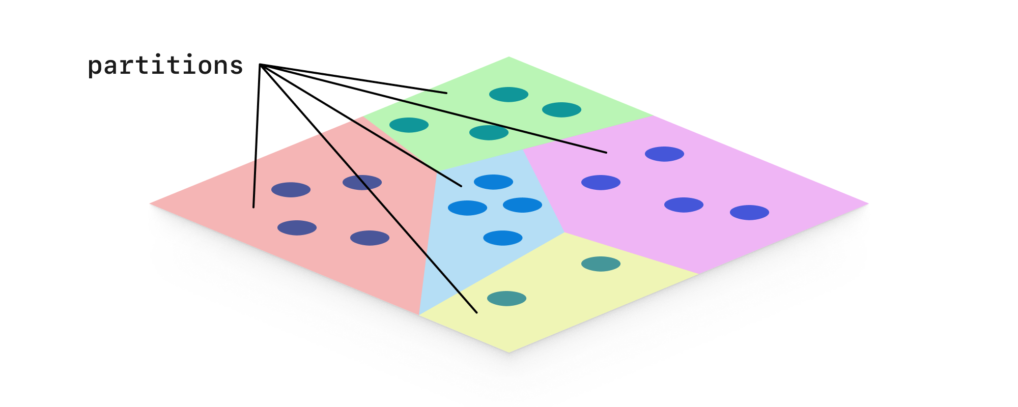

When a vector search is performed, the index finds the partition(s) that are most likely to contain similar vectors, and only performs similarity search on vectors in those.

This technique allows for much faster search compared to a full scan of all vectors, as we eliminate much of the vector data from the search early in the process. However, it might miss some similar vectors in the chunks that it skips, and therefore is only capable of performant ANN searches.

• Pros: Speeds up searches, can be combined with other methods.
• Cons: Large data sets either cause slowdown or reduced recall, or both.

Hierarchical Navigable Small World (HNSW)

HNSW is one of the most commonly implemented vector indexes in modern vector databases. This is because it provides efficient ANN search for small and medium-sized data sets, and is a widely-adopted algorithm.

HNSW indexes map every vector in the data set onto a graph, with nodes representing each vector and edges between nodes that are near each-other in the high-dimensional space.

HNSW builds multiple graph layers. The bottom layer is the full similarity graph, and each level above is a sparser version of the graph below (in other words, some nodes and edges get pruned).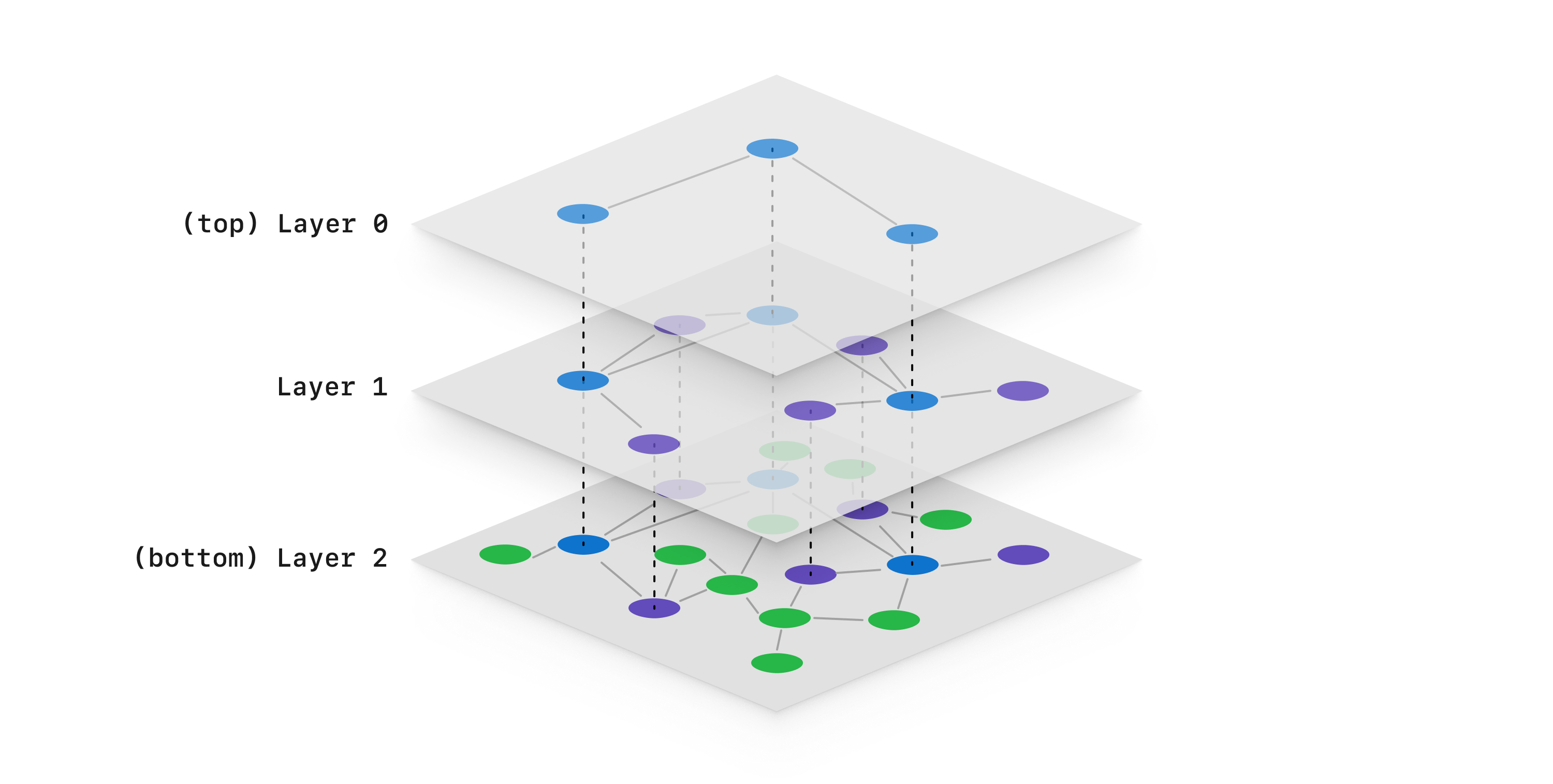

HNSW begins its search for a vector at the top layer. Since the graph is sparse, it can quickly navigate through and find the nearest similar vector. It then drops down to the next level, and continues to search for the closest vector match in that region of the graph. This process continues until it finds the closest match(es) in the lowest level.

HNSW works really well for small and medium sized vector data sets when the index can all fit in RAM. However, once the index no longer fits in RAM, performance takes a drastic hit. This is because the search on the graph produces a lot of non-sequential I/O. In memory this is fine, but this leads to poorly-optimized disk access patterns, even for SSDs.

Another downside of HNSW indexes is that they cannot be updated incrementally, so they require periodically re-building the index with the underlying vector data.

• Pros: Popular, easy to implement, fast searches.
• Cons: Does not scale well for large data sets, requires periodically re-building the index

DiskANN

DiskANN is another graph-based ANN search algorithm akin to HNSW. However, DiskANN does not use the multi-layer graph approach like HNSW does. Instead, it builds a single large graph of the vector data in several phases.

Initially, a graph node is created for each vector in the data set, and random edges are added, leading to a very "messy" graph. Then, two phases of optimization and pruning occur. The first optimization phase does significant adjustment and pruning to optimize similarity search with short edges. The second optimization phase build longer edges into the graph, allowing for faster graph traversals. This graph construction algorithm is known as Vamana.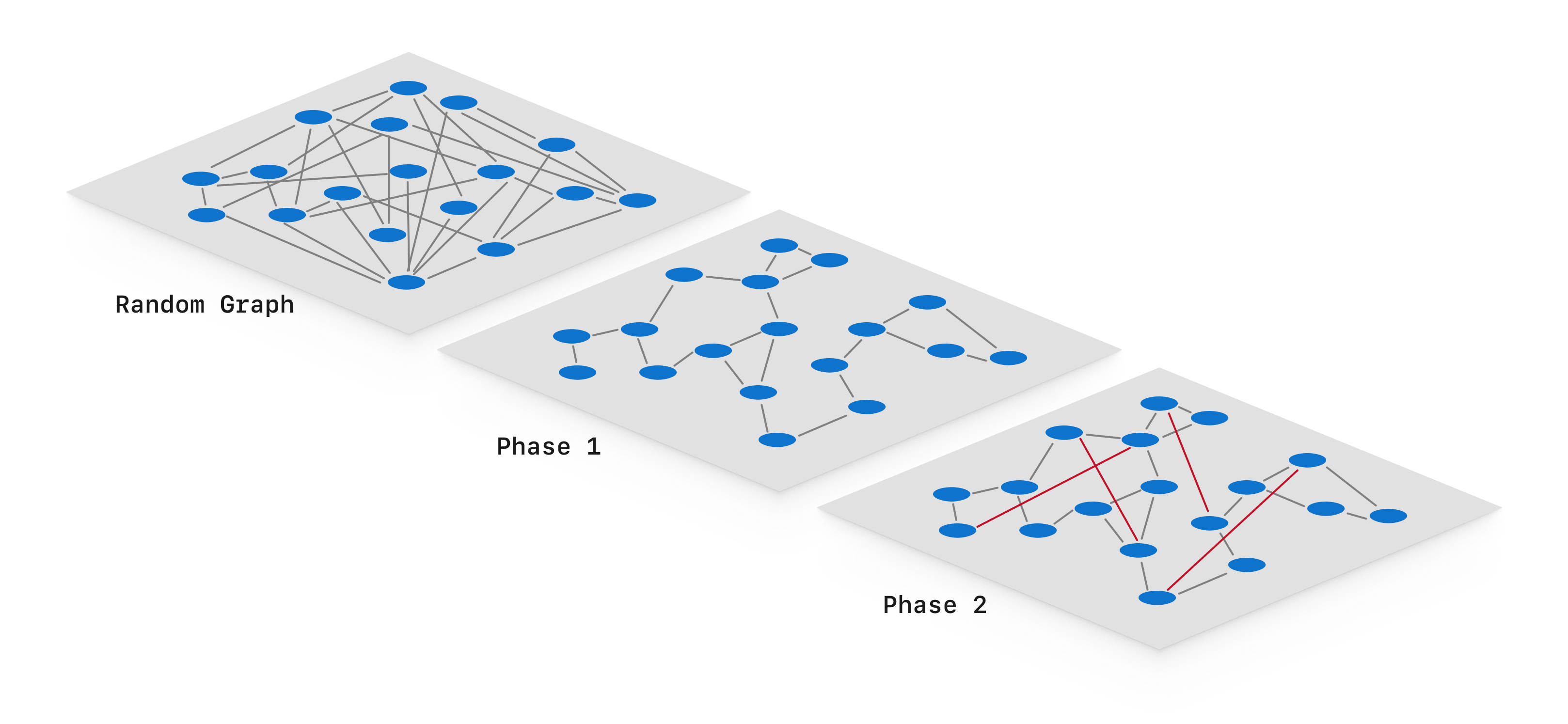

As the name suggests, DiskANN has better performance than HNSW when the index does not all fit into RAM. DiskANN uses a different technique for building the graph compared to HNSW. This technique leads to different neighbors for each node and a different memory / disk layout. When the index cannot fit into memory, this graph allows for a significant reduction in the number of disk read operations needed to fulfill a search compared to HNSW.

DiskANN scales well, but suffers from worse query performance. While it can be modified to allow incremental updates, these are not particularly efficient and are hard to map to transactional SQL semantics.

• Pros: Fast searches, scales better than HNSW or IVF
• Cons: Relies on basic graph traversal, incremental index updates are expensive

Space-Partitioned Approximate Nearest Neighbors (SPANN)

SPANN is a hybrid vector indexing and search algorithm that uses both graph and tree structures, and was specifically designed to work well for indexes requiring SSD usage.

A graph is created for the vector data, with edges representing nearby neighbors. The graph is partitioned into many small clusters called posting lists. In SPANN, nodes that are near the boundary between two posting lists may reside in multiple posting lists to help improve recall.

The full set of posting lists are stored on disk. The center-most node of each posting list (known as the centroid) is stored in a special SPTAG index, which is designed to fit in memory.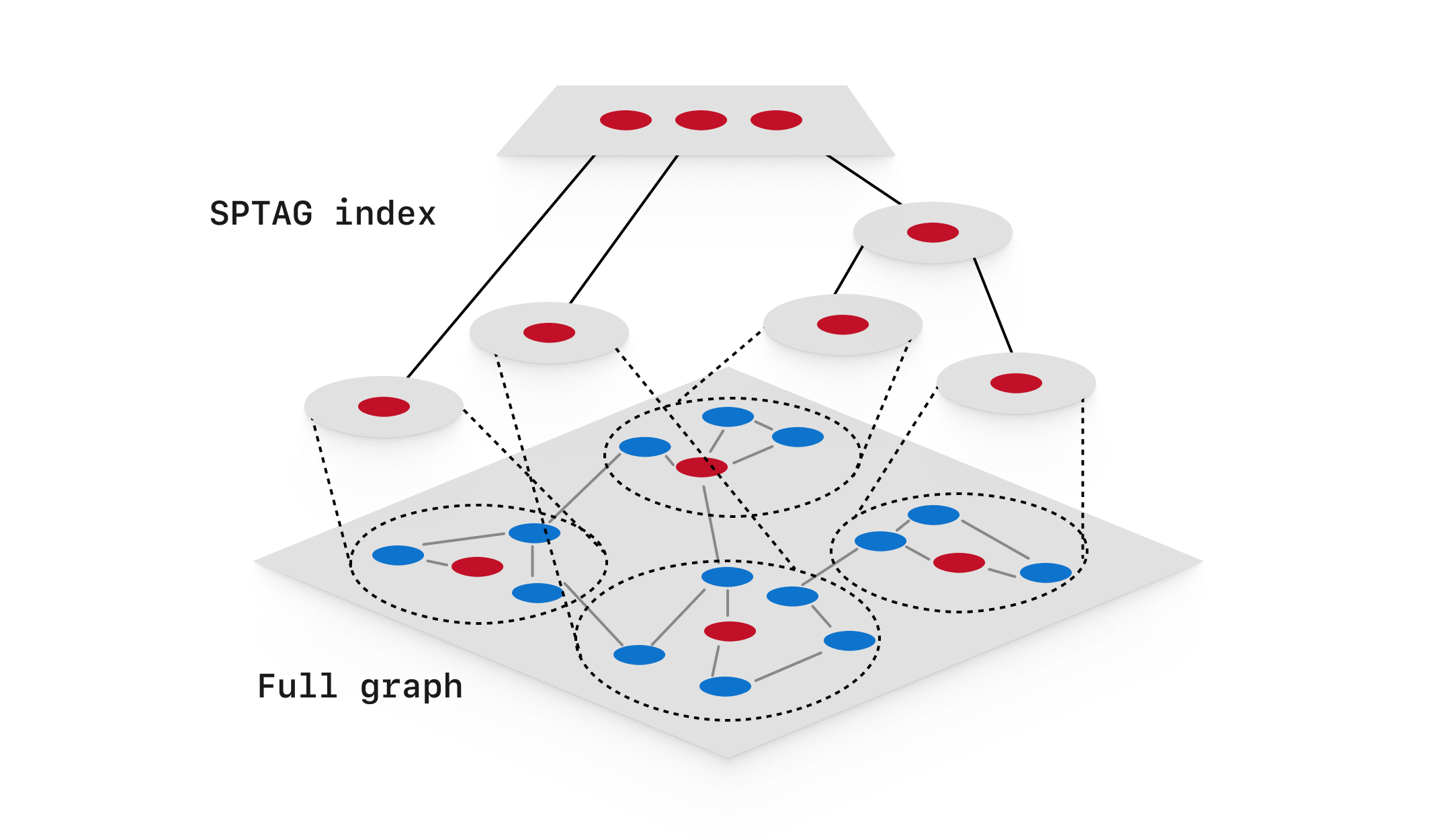

When an ANN search is performed, the search algorithm can quickly identify a small set of the nearest centroids to the search vector using the in-memory index. Then, a relatively small number of disk reads can take place to load only the relevant parts of the graph into memory, and then the search can be completed. According to the SPANN research paper, this leads to a 2x performance improvement over DiskANN.

• Pros: Fast search, scales to huge data sets, the SPFresh variant allows for efficient incremental updates
• Cons: High complexity, high disk usage because of replicated data on-disk

PlanetScale MySQL uses a variant of the SPANN algorithm for vector indexes. Though challenging to implement, we wanted to provide the best solution for our users to scale their vector data sets.

Need help?

Get help from the PlanetScale support team, or join our GitHub discussion board to see how others are using PlanetScale.