Benchmarking is hard. There are many ways to do it wrong and few to do it right.
But zooming out from any single system or harness, there are broad principles that should be applied to all benchmarking. Using these correctly makes it difficult to produce biased results.
Am I the world's best benchmarker? Certainly not. I invented the language balls, after all. But correctness and precision are important parts of PlanetScale's culture. We've spent considerable time learning the art of benchmarking, and are here to share best-practices.
Here, we're focusing primarily on benchmarking databases, but these principles apply to many domains.
Client-server architecture
Databases typically operate in a client-server model. The database server is started, accepts connections from clients, executes queries, and returns results.
To benchmark, we need a client that establishes the connections, generates queries, and takes measurements. Since both sides consume resources and we want to give the database its full share of the host server, it's common to set up a distinct server for benchmark execution.
As usual, there's a catch. This introduces latency between the two machines.
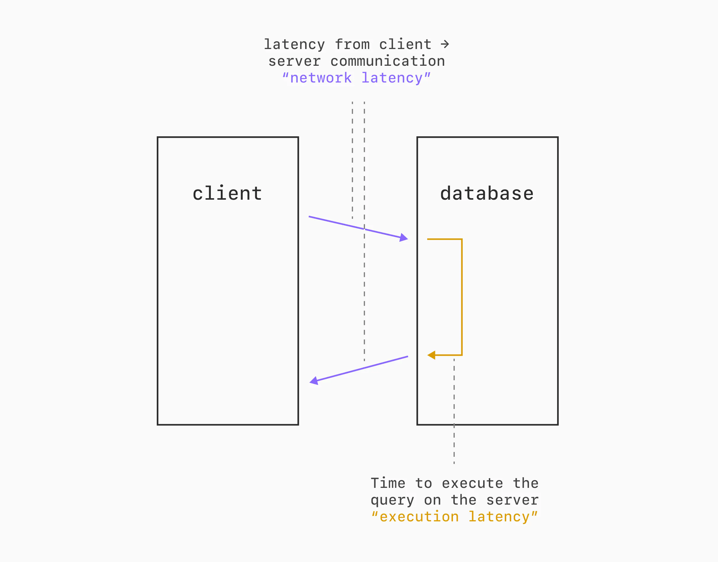
How much this skews the results of the benchmark depends quite a bit on how "far apart" the benchmark server and database server are (network latency) and how long the queries / transactions take on the database (execution latency).
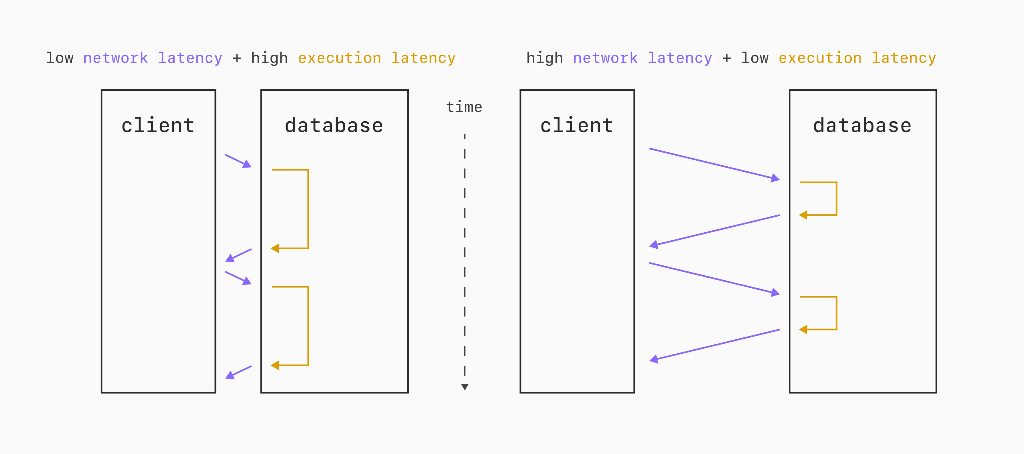
Let's consider a scenario where each query takes ~10ms to execute on the database. If the network round-trip time is 2.5 milliseconds, then we can execute approximately 80 queries per second over a single connection. On the other hand, what if the round-trip is 15 milliseconds? We've now cut our single-threaded QPS capability in ~half, resulting in 40 QPS.
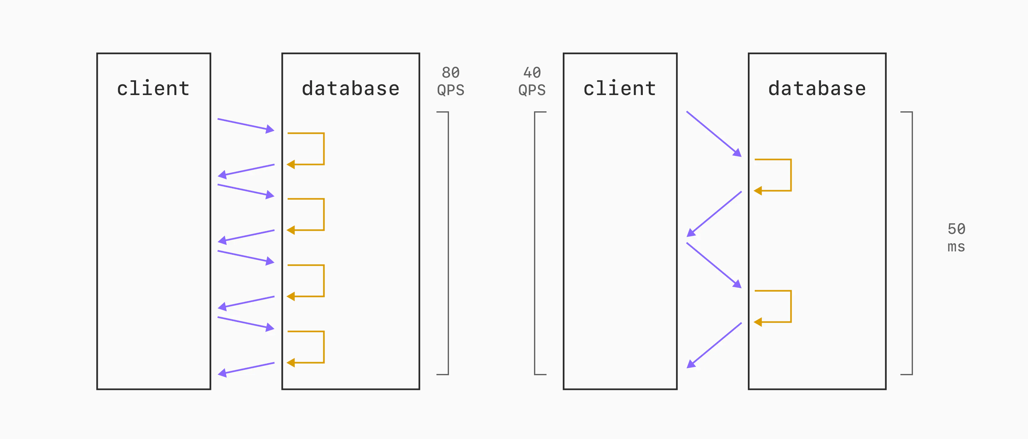
Same database. Same benchmark client. The only difference is the speed at which bytes can go over the wire between the two.
This latency variation will always have an impact on latency measurements.
It can also impact throughput. We often don't run benchmarks on a single connection. We'll do 10, 50, or 100 simultaneous connections to best utilize the parallelism of the machine and database. But if we have a fixed connection count, and are not making it dynamic to account for round-trip latency, we can end up allowing the elevated latency to hurt throughput.
Finally, you should double-check that the client server is not a bottleneck. While benchmarking, ensure that CPU and network utilization are well under their capacity. We want to be straining the database server, not the client.
Choosing resources
It's easy to make one database look better than another with an imbalance of resources. Postgres running on a 16-core server will almost always perform better than on an 8-core server.
An important prerequisite to proper benchmarking is setting up the compute, storage, and networking resources to allow for a fair fight.
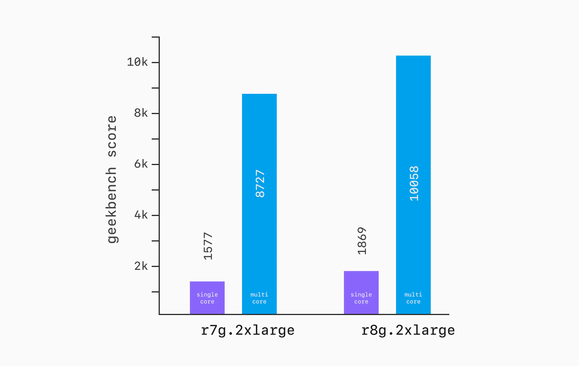
This isn't as easy as it sounds, especially when we're talking about running things in the hyperscaler clouds like AWS and GCP. For example, the Geekbench results for an AWS r7g.2xlarge are ~15% lower than the results for an r8g.2xlarge. Both have 8 vCPUs and 64 GB RAM. But move one generation newer, and there's a ~15% CPU improvement.
You might then be tempted to just use the same instance for everything, but this breaks down too. The availability of instance types varies over time, region, and database provider. In some cases, it's not possible to match.
In an ideal world, we'd run everything on the exact same instance. In reality, we sometimes have to settle for matching CPUs and RAM as best we can, and living with the differences. However, you must give this your best effort. Purposefully choosing to benchmark your product on 2025-gen CPU and then comparing to a competitor's product on a 2022 CPU, when the alternate was readily available, is intentionally misleading.
Workload
Even once we know that our infrastructure is set up sanely, there's a lot to consider for the workload we run.
The easiest way to think about this is in terms of traffic ratios.
- How many queries are hitting RAM vs disk?
- What % of the data is hot (frequently queried) vs cold (rarely queried)?
- What's the ratio of reads to writes?
All of these impact performance, especially when combined with the variations of underlying hardware.
Queries executed on a relational database often require some amount of I/O work. Writing data must always be persisted to disk. Reading data can come from the in-memory cache, or disk on cache misses.
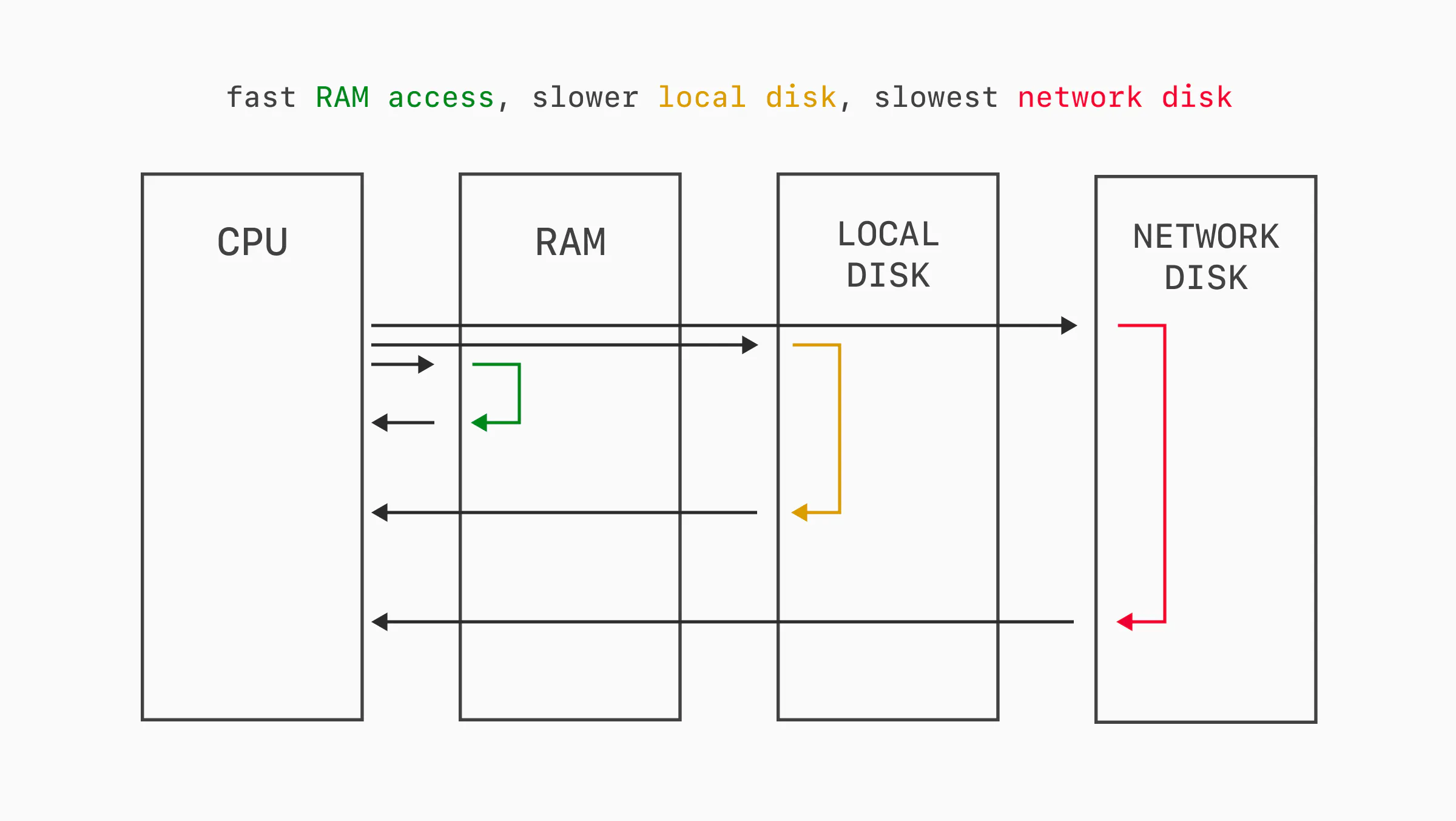
Some databases operate on local SSDs, while others use network-attached storage like AWS EBS or Google Persistent Disk. Some even take a hybrid approach. Either way, the percent of read traffic hitting RAM vs disk impacts performance due to I/O wait times.
Consider a benchmark like sysbench OLTP read-only. This is a simple, read-only benchmark that runs a handful of select query patterns repeatedly. As benchmarks often do, the data size is configurable in the preparation phase. If we run this benchmark on a server with 64 GB of RAM and a 32 GB data size, the entire data set will fit in RAM after warming. The same benchmark run with a 320 GB data size will generate significant I/O and inevitably run slower.
This is related to, but not the same as, data distribution.
Even for a fixed data size, access patterns can vary widely. The simplest examples are uniform and Zipfian.
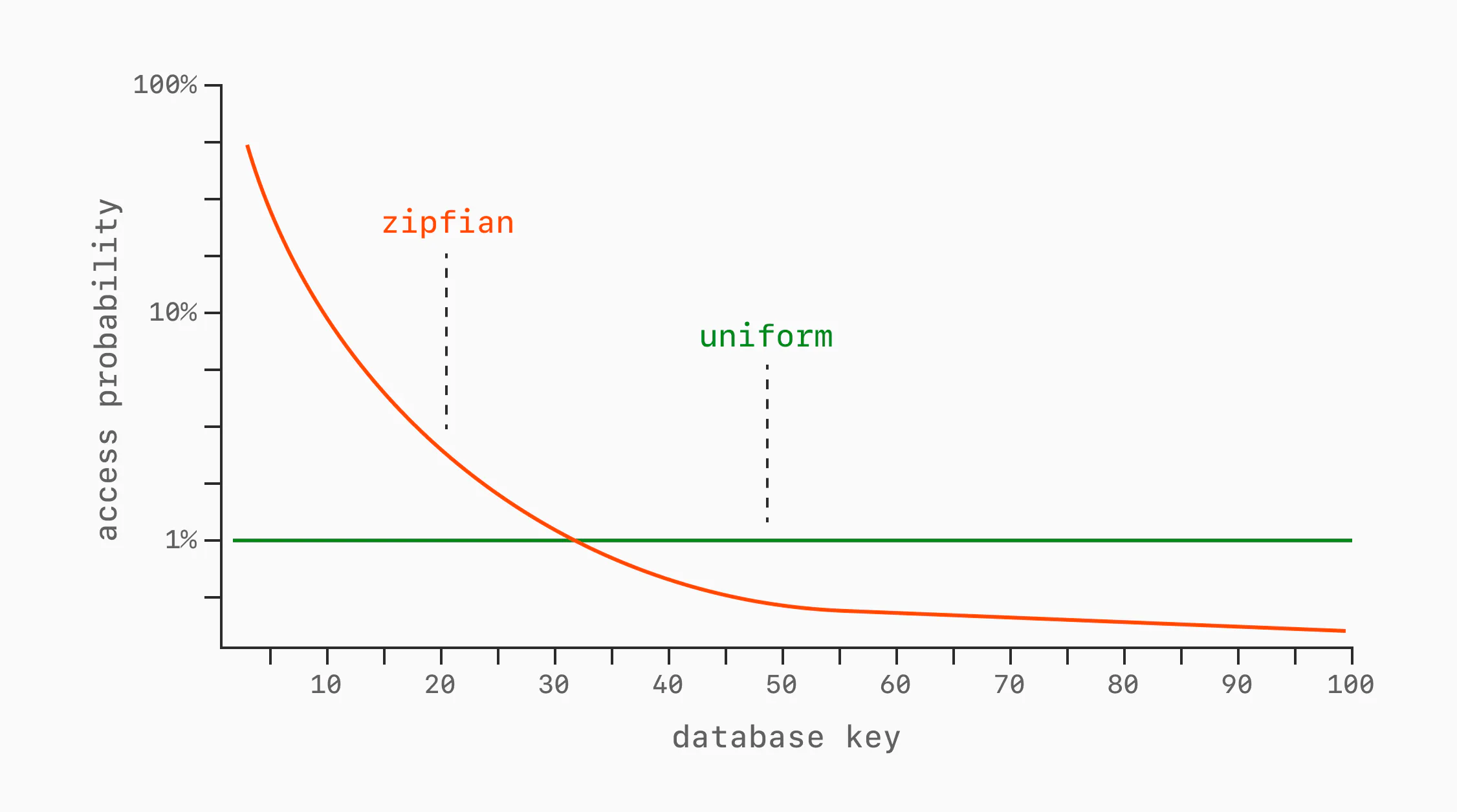
A uniform access pattern gives every row the same chance of being queried on each request. If we have 100 rows, each has a 1% chance of being read for each operation.
A Zipfian access pattern is skewed: the k-th most popular key is accessed roughly proportional to 1/k. A small number of hot rows receive a large share of requests, while most rows are accessed rarely.
These are only simple models. Real workloads often have messier shapes: recently inserted rows might be hotter than old rows, one tenant might dominate traffic, or a small working set might receive most reads for a period of time.
Which pattern the benchmark operates with significantly impacts performance, because it in turn impacts how frequently we need to access disk vs RAM and the amount of cache churn.
Closed and open loop
There are two types of benchmark workload shapes: open and closed loops.
In a closed-loop benchmark, the client sends requests and then waits for a response before sending the next.
while True:
    # wait for response
    response = send_bench_request()
    # then send next
    process(response)
We may do this in parallel across many connections, but each individual connection sends a controlled sequence of queries. A closed loop can also hide a failure mode called coordinated omission: when the database stalls, the client stops issuing new requests too, so the benchmark only records the stalled request and omits the work that would have queued behind it. This is especially misleading for tail latency, where the missing queued requests are exactly the ones that would have made p95/p99 look worse (more on latency and percentiles soon).
Open loop on the other hand has a fixed pace of sending requests, regardless of how quickly the database responds.
while True:
    # fire and forget
    send_bench_request()
    # fixed pace
    time.sleep(0.1)
This can be fixed throughout the entire benchmark duration, or vary in a controlled way:
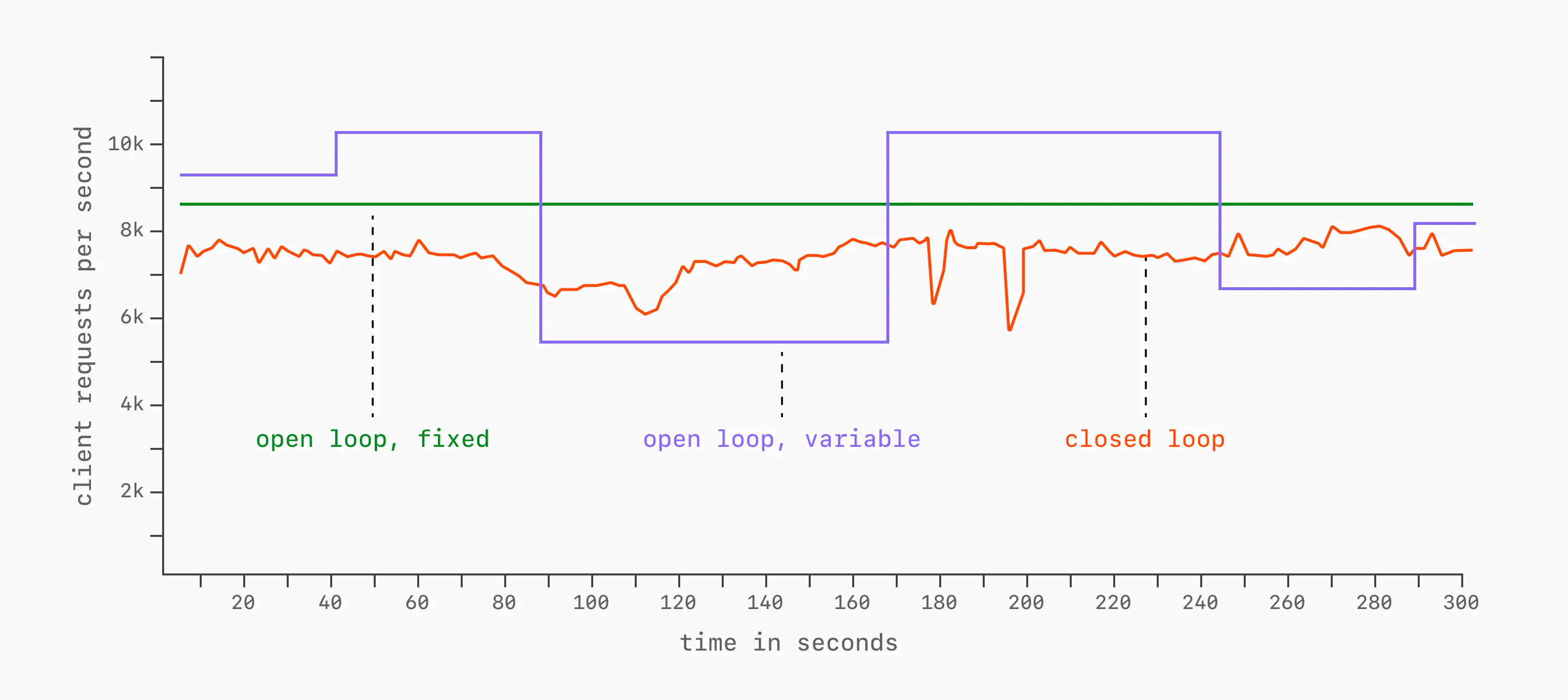
Open-loop benchmarks tend to be more realistic. In production systems, database load is applied at the rate that the clients demand, regardless of how well the database is keeping up.
Closed-loop benchmarks are more commonly seen in academic and performance comparisons, as they offer a more controlled environment for comparing things like QPS across a fixed amount of concurrency.
Both are beneficial, but they are useful for different things. Important to decide up front what the purpose of a benchmark is, then choose the type accordingly.
What to measure?
Broadly, there are two things we like to measure when benchmarking: throughput and latency. Any good database benchmark will report on both of these things.
Throughput
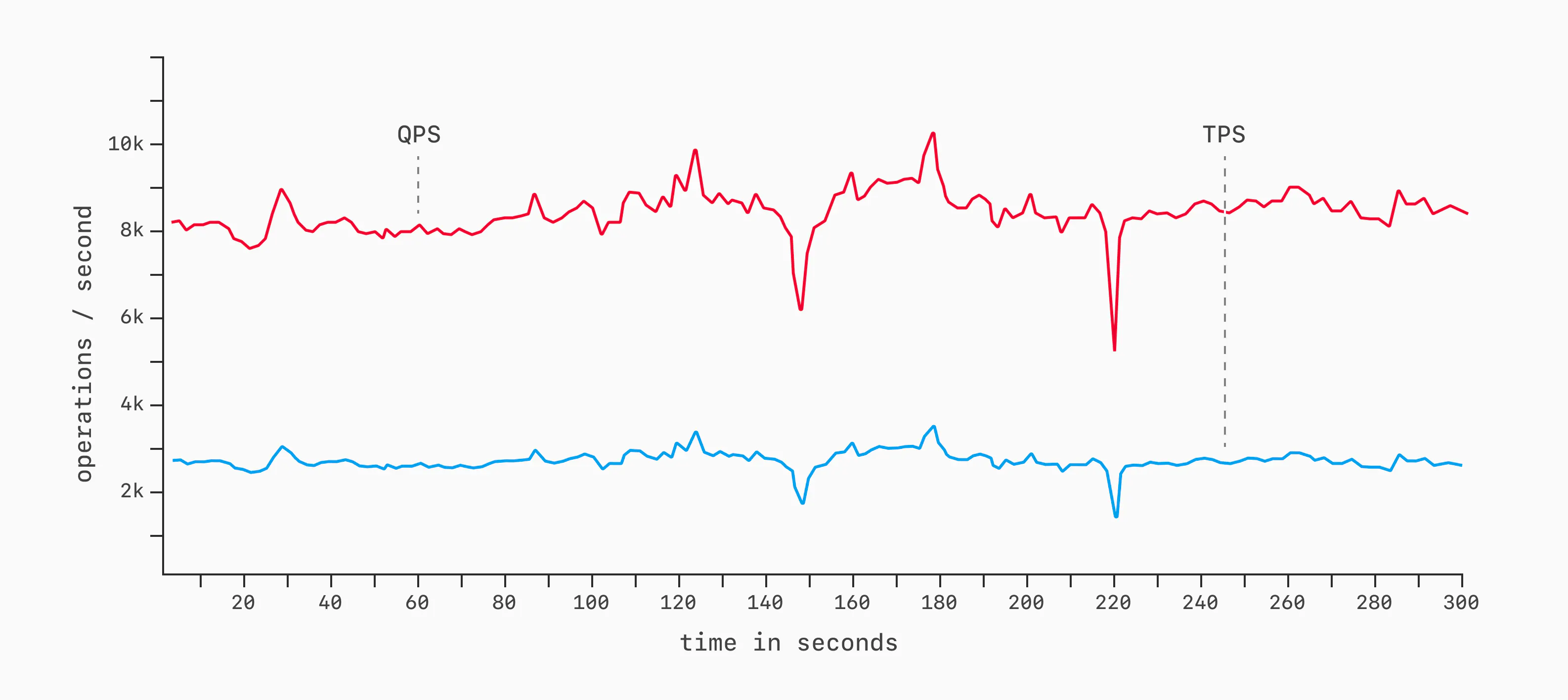
Throughput is the amount of work completed in a slice of time. In databases, the most common measures are Queries Per Second (QPS) or Transactions Per Second (TPS). For many popular benchmarks like TPC-C and TPC-H, TPS < QPS because there are typically multiple queries within single transactions. Either works fine as a measure.
To measure throughput, choose a workload, a period of time to run it for (say, 5 minutes / 300 seconds), and then execute with TPS / QPS sampling. As a benchmark runs, samples are taken of how many queries or transactions complete each second. We then display this as a graph, showing every collected data point:
A more compact way of displaying this is via a bar chart with error bars.
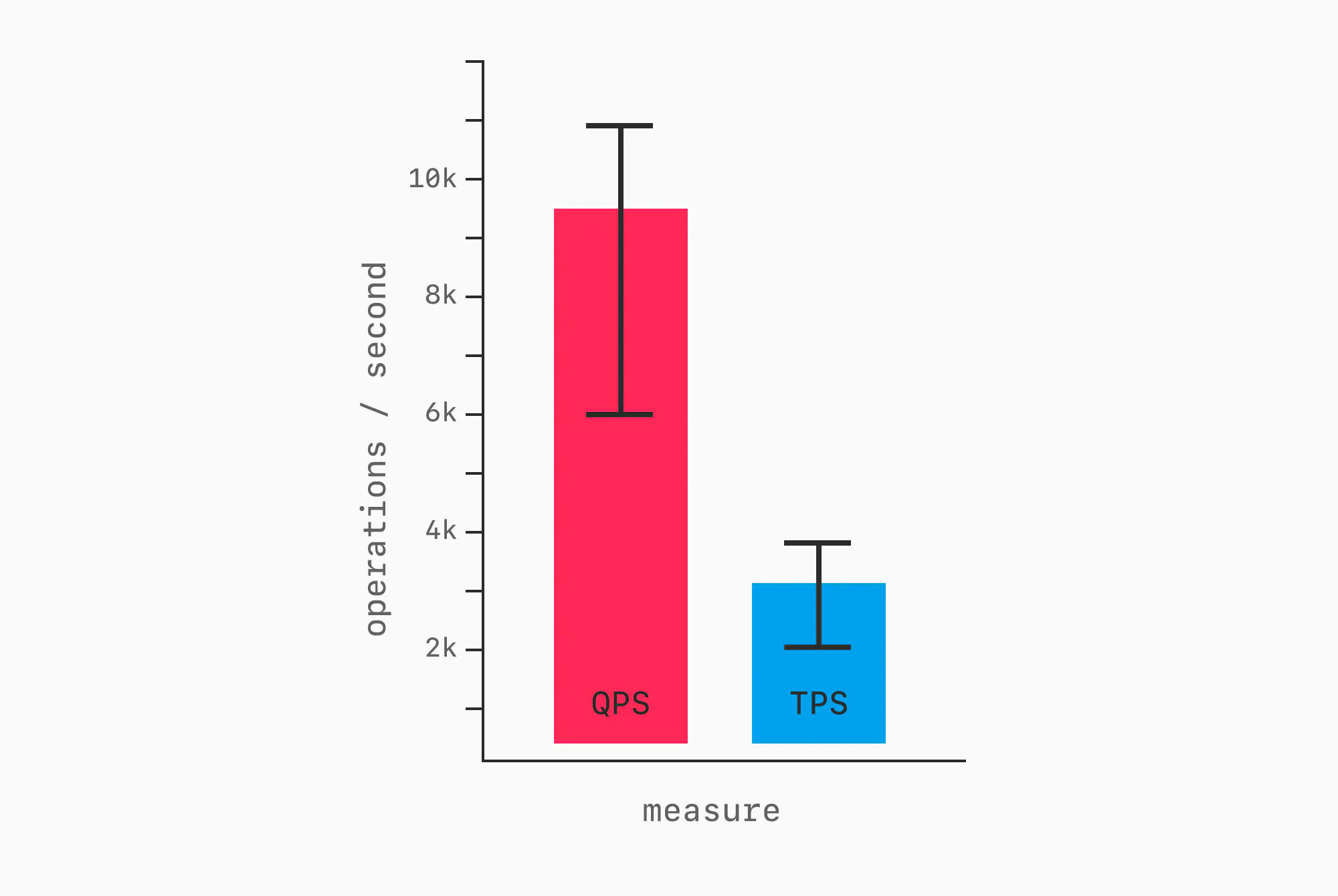
This communicates similar information in a more compact way, but it's ideal to show a full line graph, as that also better visualizes inconsistencies or spikiness of performance throughout a benchmark run. More on this later.
Error bars are only one way to summarize variance. Coefficient of variation, interquartile range, and histograms are different lenses on the same samples, each helping show whether a benchmark was stable, noisy, or hiding outliers. It's helpful to include these or provide the data so readers can compute them themselves.
Throughput only tells half the story.
Latency
Latency is the amount of time it takes to complete an operation, query, or transaction. We can look at individual latencies ("How long did this particular SELECT * FROM... take?"), but more often we assess latencies in aggregate.
The standard language for communicating about latencies in distributed systems is with percentiles over some span of time (1 second, 1 minute, etc.). For example:
- p50 - The median latency. During this time period, half of the requests executed faster than this, the other half slower.
- p90 - The 90th percentile. During this time period, 9 out of 10 requests executed faster, 1 out of 10 slower.
- p99 - The 99th percentile. During this time period, 99 out of 100 requests executed faster, 1 out of 100 slower.
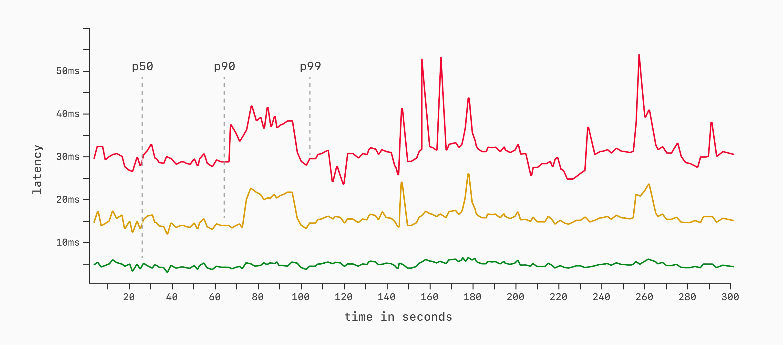
We can measure any latency percentile we want, but these are the most common, along with p95 and p99.9. When benchmarking, we typically measure one or more of these in a series of small windows over the entire benchmark period. Say, sample p50, p90, and p99 once per second over a 5-minute (300-second) execution. Then, we plot the results.
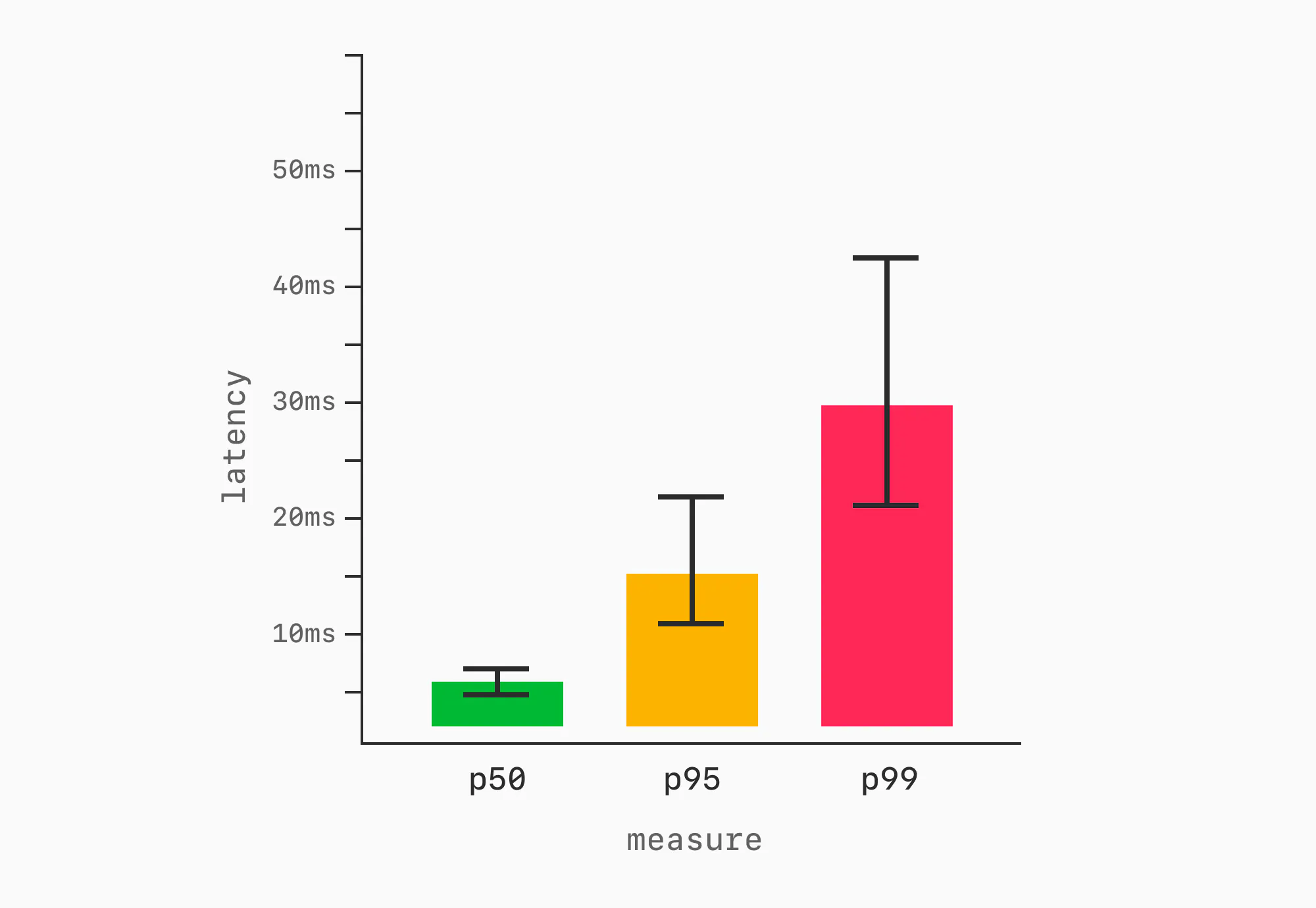
In some cases, the line graphs are overkill. As with throughput, the visual can be compressed using a bar chart showing the median (or mean), with error bars.
We now have a way of communicating both how much work we accomplished and how quickly each unit of work was completed.
Warmup
We've now settled the prep work and know what we should be measuring. Now let's get tactical. How do we ensure that we are fair when running the benchmark? There's a lot to consider for the executions themselves.
A big one is cache warmup. If we've recently booted up our database, the various caches are not full of pages (buffer_cache in Postgres, buffer_pool in MySQL). These require time and query load to warm, during which time latency and throughput will slowly be brought up to full potential.
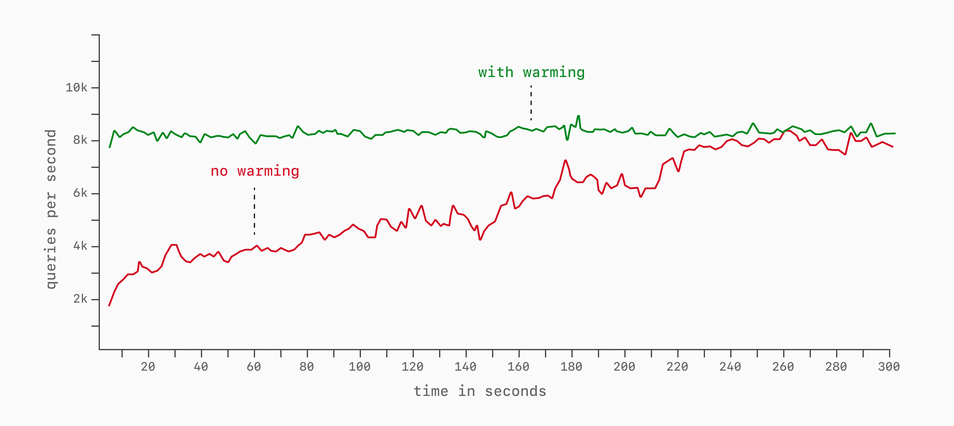
We typically run databases without measurement for a few minutes to ensure all caches are warmed before starting benchmark measurement. This ensures non-full caches and other startup costs don't impact the numbers.
Configuration
Even when warm, there are a number of configuration options that impact performance over long stretches of time. Though there are many, a good example of this is checkpoint_timeout in Postgres.
This and max_wal_size determine how frequently we need to flush table / index changes to disk (I/O checkpointing). If we set these to low / aggressive values, we may trigger it once every minute, causing regular performance dips. If we set it lax to only trigger once every ten minutes, we may not even notice it in the results of a 5-minute benchmark execution.
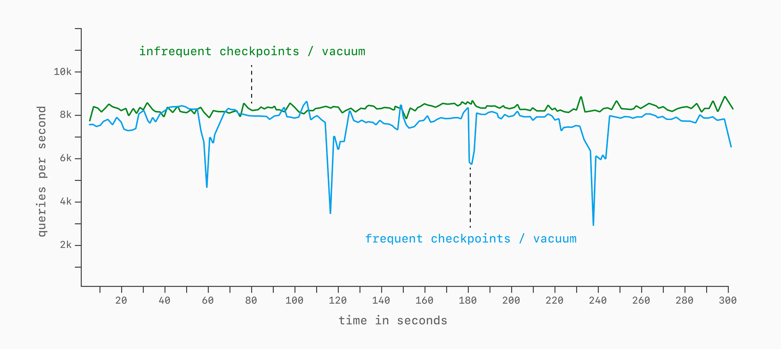
We can end up with graphs like this in these cases. But run for another 10 minutes, and we'd likely see a large performance dip on the green line.
Background jobs, I/O checkpointing, autovacuum, and other work can impact the throughput, skewing the benchmark results.
It's important to consider the impact database configurations have on performance. An identical benchmark on the same hardware can perform very differently with different tunings. DBMSs give us these tunings so we can trade off things like performance, durability, data size, and resource consumption on a case-by-case basis. It's generally best to either (a) ensure all configuration options are aligned or (b) for pre-tuned situations (like most database-as-a-service providers) leave things at the pre-tuned defaults.
(In)consistency
Another important consideration, especially in the cloud, is (in)consistency. Even with the same benchmark instance and same client machine, latency and throughput can vary from run to run. This can be due to contention on the network or noisy neighbors that are co-occupying the same hardware you are running on.
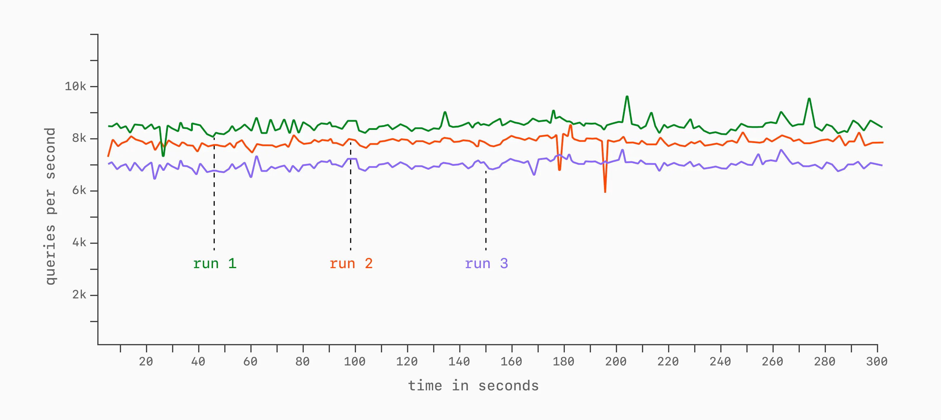
It's advisable to do multiple runs to measure consistency.
Apples to apples to oranges
The best benchmarks are the ones that compare apples-to-apples. In other words, ones that create data-driven comparisons between products that have the same or very similar characteristics and feature sets.
Examples of this are:
- Comparing 4 different Postgres configurations to determine workload suitability
- Comparing 3 different cloud MySQL platforms to determine which is most performant
- Comparing MySQL and Postgres on an identical workload (different databases, but same stated purpose)
People sometimes draw comparisons between vastly different database engines, resulting in wild claims. Things like:
- Analytics queries run 100x faster on Apache Pinot than Postgres
- Achieve 100x higher QPS on a purpose-built realtime database compared to a Postgres relational database
- SQLite latency is 80% lower than MySQL
These are comparing databases that were distinctly optimized for different purposes. It's easy to make one look better than the other, especially when cherry-picking the workload.
Don't do this. Ensure comparisons are between comparable technologies and workloads that fit the DBMS's stated purpose. The one exception may be as an internal test to determine which technology, amongst ones with vastly different goals, is best-suited for a system.
Document everything
Good benchmarks should be reproducible. Document the client and target setups as exhaustively as possible: hardware (or cloud instance type), OS, software versions, build flags, configurations, benchmark tool, exact command line, etc. After looking at the results of a benchmark, an engineer should be able to reproduce the results.
Benchmark crimes
As you can see, there's a lot to good benchmarking. Missing any one of these steps leads to bias. Some of the most common mistakes:
- Reporting only averages, without percentiles, variance, or the full time-series
- Leaving out hardware, instance type, etc.
- Measuring before the system reaches steady state
- Reporting a percentage difference without the surrounding variance
- Forgetting to check whether the benchmark client is the bottleneck
That last one is easy to miss!
If the client machine has maxed out on CPU or network connections, the graph may look like the database has plateaued. But all you've really measured is the limit of the load generator.
Go forth and benchmark
You now have an elementary understanding of database benchmarking.
When presenting results, don't stop at the numbers. If two runs differ meaningfully, offer a hypothesis for why: hardware, configuration, workload shape, cache behavior, network latency, or something else. The reader should not have to invent the causal story themselves.
Apply all these to your next round of benchmarks, and you're less likely to veer off-course.