With the advent of modern embedding models, capable of distilling the key traits of arbitrary data (including text, images and audio) into multi-dimensional vectors, the capability to index these vectors and perform similarity queries on them has become table stakes for all database products.
There has been a lot of research on this topic over the past decade, but most of it happens in a vacuum: new data structures and algorithms are designed, tested and benchmarked as standalone implementations, attempting to maximize recall and performance without taking in consideration the requirements for real-world usage of such research.
When we started the project to add vector indexes to MySQL to PlanetScale two years ago, we knew we had to implement them as a native MySQL index, because our sharded PlanetScale clusters are backed by native MySQL instances. However, we were surprised to find no existing papers discussing the trade-offs required to implement a vector index in the context of a relational database.
The majority of existing publications discuss data structures that must fit in RAM --- a non starter for any relational database! Many of them expect the indexes to be static, and indexes in a relational database very much are not. Some very few papers discuss how to continuously keep an index up to date with inserts and deletes, but they pay no attention to the transactional requirements of such operations, nor how to store them in a reliable and crash resilient way.
The lack of existing research means that we had to come up with novel solutions for all these issues in order to implement a vector index inside of MySQL that actually behaves like you'd expect an index to behave. We're stoked to be able to share our findings and our design with the community, because we believe that relational databases are the past, the present and the future of data storage, and they're long overdue for a well tailored solution for vector indexing and approximate nearest neighbor search.
Hierarchical Navigable Small Worlds
Let's start from the beginning: HNSW is a industry standard graph-based data structure that enables very efficient approximate nearest neighbor search. When discussing HNSW, it’s crucial to focus on the key word “data structure”. Just like a B-tree is not a relational database, an HNSW graph is not a vector database. There’s a big gap of functionality between the data structure and a fully featured software product that can be used by end users. Nonetheless, many standalone vector databases and embedded vector indexes in relational databases are based on this data structure, and for good reasons. HNSW has been widely adopted because it has many advantages: it has good performance and good recall, and it is simple to implement and maintain.
Like all ANN algorithms, HNSW works for vectors of arbitrary dimensionality. Even though in real-life systems the dimensionality of these vectors is huge (OpenAI embedding vectors have either 1536 or 3072 dimensions!), in this blog post we’re going to use three-dimensional vector data sets, because they’re by far the easiest to visualize and understand. If you’ve somehow managed to escape this cursed prison of flesh and currently exist as an eternal being outside of time and space, please feel free to project the following examples into whichever dimensionality seems more intuitive according to your understanding of reality.
HNSW is a multi-layered graph data structure. Every vector in the indexed dataset maps to one node in the graph, and each node of the graph may exist in one or more layers. The bottom layer of the graph contains all the nodes, and every layer above it contains a strictly decreasing subset of them. For each node in the graph, a bounded amount of edges K links it to the nearest K vectors in the N-dimensional space.
Let’s see an example of the graph and its relations:
On the top, you can see the vectors laid out in the three-dimensional space. On the bottom, you can see the actual graph. Each node in the graph maps to a vector in the 3D space (hover any of them to see the relation!), but keep in mind that the position of the nodes in the graph is arbitrary. We’ve arranged them like that so their relationships are clear and their edges don’t overlap, but the only positioning that really matters is for the points in the 3D space; the distances between these 3D points are what guides our ANN search.
You can also see how from this very simple graph we have a solid starting point to perform ANN searches. If we have a vector V as the target for our query, we can find a node in the graph that is close to V in N-dimensional space. By traversing all the neighbors of that node, we find K vectors that are close to our target. We can then compute the distance between V and each of those vectors and sort these distances to obtain a good result for our ANN query.
The problem is now finding that node in the bottom layer that is close to our target vector. This is where the multi-layering of the data structure comes in. The bottom layer of the graph, as we’ve seen, contains all the nodes, but every subsequent layer on top of it contains a random subset of all the nodes below. How many layers are there in the graph then? It depends on the total node count, but the goal is constructing this multi-level graph so that the graph on the top level is quite sparse and fully connected.
Since the nodes at all layers of the graph follow the same connection rule as the bottom layer (each node has edges up to K nodes that are actually nearby in the N-dimensional space), this produces an efficient approach to get progressively closer to our target node in the bottom layer.
We start on the top layer of the graph. Since the layer is fully connected, we can pick an arbitrary node as a starting point and then traverse all its neighbors looking for the one whose vector is closest to our target vector. When we find such node, we descend one layer through the graph. We now perform the same operation on the same node, but we have a larger set of neighbors because each layer of the graph is denser than the previous one. With this approach, every time we go down a layer we’ve found a node that is closer to our target vector, until we finally reach the bottom layer.
Throughout this descent, we keep a priority queue and a set of all the vectors we’ve seen and their distances. The set ensures that we don’t visit the same node twice, and the priority queue incrementally stores the result of our ANN query. Once we’ve visited the K closest neighbors in the bottom layer, the top K nodes in our priority queue, sorted by distance, are the output of the algorithm.
I hope this breakdown was useful! As you’ve seen, one of the key advantages of HNSW as a data structure is that it’s very easy to understand and very easy to implement. But this simplicity comes with its fair share of shortcomings.
HNSW in a relational context
In a vacuum, HNSW is often the king of benchmarks. If you build a properly optimized HNSW graph in memory, and all of it fits in RAM without paging, it’s very hard to beat both the recall and the performance of this data structure. But here we’re talking about building a vector index for a relational database, and we have to consider technical constraints that make HNSW much less appealing.
First and foremost: the datasets that are often stored in a relational database do not fit in RAM. One of the core design choices for our implementation of vector indexes in MySQL is that we need to support indexes that are significantly larger than RAM, because that’s what users usually expect from a relational database. It’s extremely frequent to have terabyte-sized MySQL instances running in a host with just hundreds of GB of RAM, and the same applies at smaller scales (hundreds of GBs of data on-disk in a MySQL instance with 32GB of RAM). InnoDB, the default storage engine for MySQL, manages swapping in and out data from disk into memory to ensure that the system performs well despite this mismatch between available memory and total size of the working set.
Secondly, HNSW is a mostly static data structure, very much unlike the behavior of your average database table. A relational database operates under a constant stream of inserts, updates and deletes, and has been designed to perform all these operations with good performance and following a set of data consistency constraints: atomicity, consistency, isolation, durability. None of this applies to HNSW out of the box unless you put a lot of thought into making this apply!
There are roughly two ways to make this happen:
- You can try to store the graph inside the database. Although this solves the transactionality issues, this is also, broadly speaking, a bad idea. Relational databases are not graph databases, as anybody who’s ever tried to store a graph as SQL can attest. The data model by itself is straightforward, but actually running algorithms on the data is a world of pain, because every hop through the graph requires one look-up on the B-tree, and these look-ups often have a dependency chain: you cannot perform the next lookup in parallel because it depends on the previous one.
- Alternatively, you can reserve enough memory upfront and keep the graph in-memory. This gives you the best possible performance by far, but it requires a lot of nuance when it comes to maintaining the index and its transactional guarantees.
We know that the performance and recall of HNSW is at this point expected for many AI-related workloads, particularly those with small datasets, so we’ve made sure that our implementation of Vector Indexes in MySQL for PlanetScale supports fully in-memory HNSW indexes with transactional guarantees, with high performance and 99.9% recall if you’re willing to support the trade-offs: you need to allocate enough memory to vector indexes in your database to fit your whole vector dataset, and incrementally updating these indexes is very expensive.
But we also know that in many workloads, allocating so much memory up-front for vector indexes is not a reasonable trade-off, so we’ve made a significant effort to design a new kind of hybrid vector index that really behaves like you’d expect an index in a relational database to behave.
Our design philosophy
A vector index is very different from any other kind of index used in a relational database because it’s approximate. You’re not expecting the results of any query that uses the index to be 100% accurate, and this makes it very appealing to start cutting corners when it comes to the consistency and availability of the data. When a user inserts a thousand vectors into a table in a single database commit, this will make the commit an expensive operation, and it would be very easy to play it fast and loose when updating the vector index for that table accordingly. This is approximate nearest neighbor search after all, isn’t it? If you do a SELECT after that commit and a few of the vectors are missing, hey, that’s recall loss. Shit happens. The vectors will appear in other queries, eventually.
We don’t think this is a reasonable approach when implementing a vector index for a relational database. Beyond pragmatism, our guiding light behind this implementation is ensuring that vector indexes in a PlanetScale MySQL database behave like you’d expect any other index to behave. This means that if you’ve just committed a thousand vectors, the next SELECT will consider all of them for a similarity query, even if not all of them are returned because the recall is not perfect. This means that if you abort the transaction with the thousand vectors, they will not appear in the index at all. And this means that this all applies always, whether your database is in the process of failing over or recovering from a crash.
This engineering philosophy comes with a clear set of trade-offs: the disk-backed, transactional indexes of our implementation are necessarily slower than any other implementation that operates fully in-memory, including our very own HNSW indexes which you can always opt-in into. After all, our larger-than-RAM indexes store their actual vector data inside of InnoDB, which is a fully fledged ACID storage engine. This is not an engineering decision we took lightly; we arrived at this design after a lot of research — looking at existing databases and at the needs of our customers. But it is a decision we’re happy with. Let’s look into it in detail.
PlanetScale Hybrid Vector Search
Like most vector index designs used in production systems, ours is a hybrid index. This index is composed of two layers: an in-memory HNSW index that stores vectors as a graph, based on our transactional HNSW index implementation, and an on-disk index that stores vectors as posting lists.
The in-memory HNSW index is what we call a ”head index”. This data structure contains a subset of all vectors of the full index. The default is 20%, although you can tune that to be smaller at index construction, trading off reduced memory usage for worse recall. The remaining 80% of the vectors are stored as posting lists (i.e. just raw binary blobs where the vectors appear one after the other) in MySQL’s default storage engine, InnoDB.
The head index contains a random sampling of all the vectors in the dataset, each vector being a "head" or "centroid". For each head in this index, a posting list is generated containing K vectors which are nearby in the N-dimensional space. The value of K depends on the dimensionality of the vectors; the goal is ensuring that all posting lists are of similar size in bytes and that they're never large enough to slow down InnoDB lookups for their blobs.
This design is similar to the one proposed in SPANN: Highly-efficient Billion-scale Approximate Nearest Neighbor Search, but with some key differences. The original paper from Microsoft Research proposes several approaches to construct and store the head index, based on alternative graph-based data structures such as BK Trees and K-D Trees. It is not clear to us why HNSW was not evaluated in the paper, but in our experiments, an optimized implementation of HNSW beats these other data structures in every possible metric (performance, recall, construction time), so our hybrid indexes use HNSW for the head index.
Similarly, the SPANN paper discusses a complex clustering algorithm based on BK Trees to select the subset of vectors that will belong to the head index, but after thorough testing with real-life datasets, we concluded that random sampling provides good results in practice: when the dataset is large enough, the law of large numbers ensures that our random sampling is representative, whilst for small datasets, a slightly unbalanced head index has little effect on the total recall of the index. Most importantly: by sampling randomly from the original dataset of vectors, which are stored directly in the user’s table in InnoDB, we can construct larger-than-RAM indexes requiring only up to 30% of the memory size used by the dataset.
Once constructed, the operational index only maintains allocated 20% of the total dataset (i.e. the size of the head index), fulfilling our first technical goal. With this design, the vast majority of the vector data is stored as posting lists and managed by InnoDB. You do not need enough memory in your database instances to contain the full size of your indexes, as only 20% or less needs to be reserved for queries to succeed.
This design acts as a solid starting point to provide ANN queries on a larger-than-RAM vector dataset. The subsequent challenge now is ensuring that the index can remain fresh, i.e. that it can be continuously updated in real time while serving queries with high recall.
Inserts
The high-level logic for inserting new vectors into the index is as follows: we perform an ANN search on the Head index for every vector we’re trying to append, to find the posting lists where it belongs. Note the plural here! A single vector can land in one or more posting lists, because vectors that are too close to the edge of a cluster will be replicated in neighboring clusters to increase recall. Then, we insert a copy of the vector on each of the posting lists.
So far so easy, but the devil is in the details. What does it mean to insert the vector in a posting list? As we’ve seen, posting lists are serialized blobs stored as values in InnoDB, where their key is the vector ID for the centroid of that specific cluster of vectors. Hence, inserting another vector into the cluster means appending it at the end of the serialized blob. This is a very simple operation in theory, but very complex in the context of a relational database.
If we were to write this operation as a normal SQL query, it’d look something like this:
UPDATE vector_index_table
SET postings = CONCAT(postings, :new_vector_data)
WHERE head_id = :target_head_id;
This is because our posting lists are stored into something that looks a lot like a vector_index_table, just lower level: we use InnoDB’s B-tree API directly to read and write our postings. If you’re unsure what a B-tree is or how it relates to storing data in a relational database, my friend Ben has a very good post in this same blog called “B-trees and database indexes” which you should definitely check out. Seriously, I mean it, it’s very good and it has a lot of fun, interactive animations. So go forth and read the things and click the buttons, I’ll wait.
Back already? I hope you’re enjoying your newfound or refreshed knowledge about B-trees. Ben’s blog talks a lot about keys in the B-tree, so let me expand it by talking briefly about values. One major shortcoming of B-trees in the real world is that updating their values can be very expensive. Changing the value of an integer column, for instance, is perfectly fine because all integers take up the same space on the leaves of the B-tree. But changing the value of a BLOB can be a pain in the ass. Blobs can be stored inline in the leaves of the tree, or out-of-tree, where the actual content of the blob is stored in several dedicated InnoDB pages and a pointer to these contents is stored in the B-tree (these are called LOBS in InnoDB, short for Large blOBS). But regardless of their location, the situation is the same: adding data to the end of a blob is just not possible, because after each blob there’s always… huh, something else. Maybe another blob, maybe another row in the B-tree. But there just isn’t space!
So, breaking down the simple SQL query which we’ve just seen above, it turns out that it’s not so simple after all. That CONCAT operation is not “appending” data at the end of the existing blob, it’s creating a brand new blob by copying the existing one and leaving enough space at the end to place the new vector data. The old blob is then left to rot in the B-tree — hopefully it’ll get garbage collected for further inserts in the future. And to make things worse, this is a two-step operation: we must first read the existing blob, then write back a brand new one, so the only way this would be safe to do in practice is by acquiring a row-level lock for the whole operation. InnoDB in fact does this implicitly when running such an SQL query.
In summary: the performance implications of appending data at the end of our posting lists are atrocious. Clearly the original SPANN paper did not take into account the characteristics of a relational database when designing their Insertion algorithm, so we’ll have to come up with a plan B. Let’s start by the most obvious place: how do they actually perform Inserts in the SPANN paper? Do they do it efficiently? And if so, can we copy that design?
Efficient updates on top of LSM trees
The answer lies in the dastardly cousin of the B-tree: the Log-Structured Merge Tree (or LSM tree for short). Unfortunately Ben hasn’t yet gotten around to writing the blog post about LSM trees, so you don’t get to click any more buttons while learning about this topic. Sorry! I hope you’ve at least heard of them (you can peruse the Wikipedia entry on the topic if not), but I’ll give you a quick rundown:
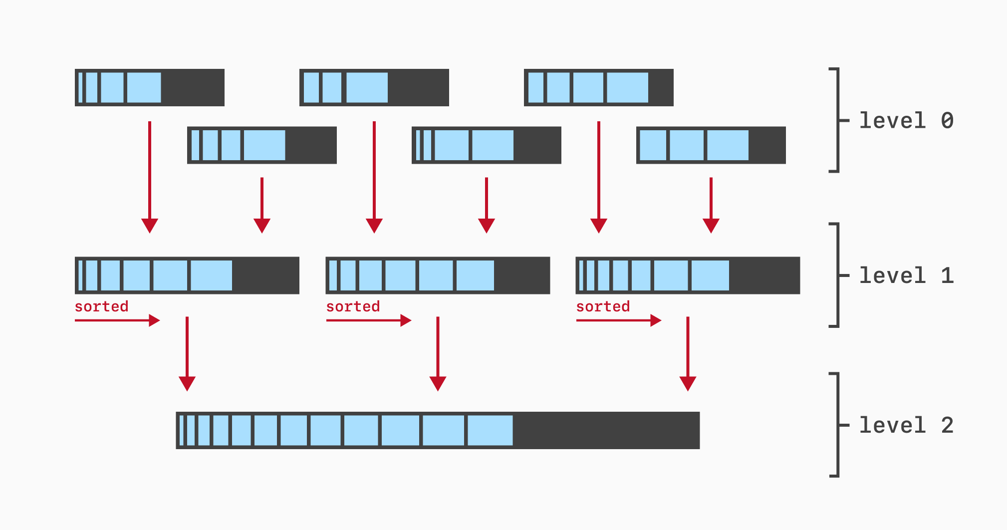
LSM trees maintain key-value pairs (like B-trees), but they’re a hybrid data structure. The K/V data is stored in two places: an in-memory table, that is optimized to stay in memory, and a set of on-disk tables, that are optimized to stay on disk. The key idea behind the performance characteristics of an LSM tree is that data is always flushed in batches between each layer. For instance, once the memory table grows large enough, it is flushed into a single table on disk, which can be written sequentially (this is very fast!). Once there are too many tables on disk, they’re all aggregated into fewer larger tables, which are once again written sequentially to disk. This process, called “compaction”, runs continuously to ensure that there’s a minimal amount of tables on disk.
We can gather some interesting performance insights already with this basic knowledge about LSM trees: write performance must be very good because data is always written sequentially (unlike with a B-tree, which writes data all over the place). Lookup performance must kinda suck, because to look-up an individual key you’d often need to check several tables, both in memory and on-disk (in real-world implementations, this is fixed by using bloom filters to quickly figure out which tables can contain a given key). And range scans must really suck because, well, data is not globally sorted (in real-world implementations, this is fixed by not doing range scans and using a B-tree instead, heehee).
Now, how does all of this mix with the SPFresh paper? We’re getting there. It turns out that the efficient Insert in SPANN vector indexes was designed to be performed on top of LSM trees. That kind of makes sense – we’ve seen LSM trees are very good at writes, but there’s quite a bit more to it. LSM trees are actually uniquely good at the exact same problem we’re trying to solve when inserting data into our vector index: appending a value at the end of an existing value!
Here’s how this works: usually an update for a key/value in an LSM tree means just adding a new key/value pair to its memory table. Once this memory table is eventually flushed to disk and merged with other tables that were previously on-disk, the compaction algorithm will notice that the new key/value pair we’ve inserted is newer than the one that was sitting on disk, and will drop the old one during compaction, leaving only the new.
But there’s this super-cool magic trick you can do with a key/value pair in a LSM tree, which is tagging the pair with a special flag (most implementations call it a “merge” flag) when inserting it into the memtable. What happens then is that the compaction algorithm can see the “merge” flag and instead of considering the value for the key as newer, and replacing any existing on-disk values, it just… merges it! When flushing the new table to disk, it first flushes the old value, and then the new one. We get a lot from this simple trick. The append no longer needs to remove the old value, and it doesn’t need to insert a brand new one either; you just insert the new vector data into the memtable and eventually they’ll be merged on disk. Most critically, you don’t even need to read the old value at insert time so you can append the new data at the end; the concatenation will be performed atomically by the compaction algorithm. So there’s no locking involved during inserts either.
Clearly, it seems like LSM trees are a match made in heaven for this specific vector index algorithm. They just provide an incredibly efficient way to continuously perform insertions that append data to existing values, which is exactly what we want to do here. So this brings our next question: can you use a LSM tree in a relational database?
The answer is a resounding YES. Meta (the company formerly known as Facebook) develops an open-source LSM-based storage engine for MySQL called MyRocks, based on RocksDB, the state-of-the-art when it comes to LSM implementations. However, it’s not as easy as just picking up MyRocks and building our vector indexes on top of it. A big constraint of storage engines in MySQL is that indexes and their tables must use the same storage engine. This is a problem in practice because MyRocks comes with a large set of trade-offs when it comes to performance — the ones we’ve just discussed. It is extremely write-optimized, and point look-ups work quite well, but range scans are very slow.
Unfortunately, the average CRUD app running on PlanetScale just performs better on InnoDB than on MyRocks, and forcing users to switch storage engines from InnoDB to MyRocks if they want to use vector indexes seemed like an unacceptable barrier to adoption.
Because of this, we’ve developed an alternative approach to emulate LSM compaction on top of InnoDB, enabling very fast inserts when building vector indexes without requiring switching storage engines.
Emulating LSM compaction in a B-tree
The approach we’ve employed in our InnoDB-based index is not complex, and yet provides very good results in practice. Instead of structuring our B-tree index for posting lists as a simple mapping between head vector IDs to posting lists, we’ve constructed a composite index. This is an essential feature of all B-trees for relational databases, including InnoDB: it means using more than one value as the key for the index, and since a B-tree is always sorted, it allows us to perform queries on a prefix of our keys, instead of having to match the keys exactly.
Our composite index uses key a tuple of (head_vector_id, sequence), where sequence is a table-local strictly increasing sequence number. With this, we can approach posting list updates in a very efficient way: we insert a new row into the table with the head_vector_id we’re appending to and the next sequence number for the table. This is incredibly friendly to the B-tree compared to the naive approach of looking up the head_vector_id, appending the data to the existing posting list, and then writing it back to the B-tree. It gets rid of the initial lookup altogether, and consequently of all the locking!
This optimization when updating posting lists comes with a price at query time, but it happens to be quite small in practice. When we’re looking up the posting list for a specific head_vector_id, it no longer becomes a point query on the B-tree; we now must perform a range scan for all rows that begin with head_vector_id. The actual posting list is the result of joining all the posting list values in each row together. Fortunately, B-trees are very good at range scans, because adjacent keys are stored next to each other in the pages.
The other problem with this approach is that you can end with a lot of rows on your posting tables, slowly degrading the performance of index queries. Do not fear! This is also solvable. In fact, continuously adding data to the vector index comes with many side effects that degrade its recall and performance, but they can all solved with a similar and elegant approach. Let’s look at these issues one by one.
Splits
There’s one essential way in which this kind of vector index degrades when continuously inserting new data into it. We’ve seen how to efficiently append vector data to our posting lists, but although each individual insert happens very quickly, this is not an operation we can continuously perform. If we keep appending data to each posting list in the index, eventually the postings will become large enough to affect query performance!
One of the key invariants for our index design is that query performance must be bounded, regardless of the size of the index, which means we must prevent any single posting list from growing too large. To accomplish this, we’ve implemented the key idea from a follow-up paper from Microsoft research: SPFresh. This paper expands on the original SPANN index by layering the LIRE protocol (Lightweight Incremental Re-balancing). LIRE is composed of a set of small incremental operations which are continuously performed in the background in order to maintain the key properties of the index and ensure high recall and good query performance.
The most important of these operations is the Split. A split may be triggered during any insert operation to the index, whenever we detect that a posting list has grown too large after appending new vectors to it. Like all LIRE operations, the split is triggered to run in the background; it does not happen as part of the commit that appended the vectors. This means that the vectors become visible for queries as soon as the commit is finalized, but that the posting list that contains them and which is now too large, will soon be picked up by a background job and optimized.
The logic behind a split is quite self-explanatory: we gather all the vectors contained in the large posting list and split them. The original LIRE protocol in the paper always performs this split using K-means clustering to detect two new clusters. The centroids for these clusters are then inserted into the Head Index, and the original posting list is written back to InnoDB as two posting lists of very similar sizes, each keyed by one of the new Heads. For our implementation, we’ve improved this process further by allowing the K-means clustering to split the posting list into K different clusters, where K is calculated based on the expected size of each posting list. During normal operation, this K is often 2, but when the index is under high insertion load, a single posting list can grow very large before its corresponding background job gets to pick it up for splitting, so being able to immediately split it into multiple smaller postings is an important optimization.
By continuously performing splits whenever an individual posting list grows too large, we ensure that the performance of index queries remains stable. But these splits actually have a negative and counter-intuitive impact on the other key property of the index: they degrade its recall.
Reassignments
Consider this three-dimensional dataset. We can see three clusters, each keyed by a different Head from the HNSW index. The largest of these clusters is actually too large compared to the other two (it just contains more vectors), so it has been scheduled for splitting.
The result of the split is as we’d expect: two new heads have been created and inserted into the head index, and we now have two smaller clusters, each of them stored in a separate posting list. But pay close attention to the highlighted vectors in the newly formed clusters. Can you see what’s off about them?
Hovering over the highlighted vectors gives you a big clue, as you can see the distances to the head of their cluster and to all nearby heads of other clusters. It turns out that since the centroid of the original cluster has been split into two, some of these vectors are no longer assigned to their nearest centroid in three-dimensional space! This breaks the NPA (nearest partition assignment) invariant of the index.
This is an unfortunate side-effect of performing a split that only considers one posting list of the index. When clustering all the vectors in this posting list, the K-means result yields optimal results locally, but if we start considering other surrounding vectors, we see that their distances to the new centroids are a local minimum. Hence, performing splits over and over again eventually degrades the recall of the index, because it places many vectors in posting lists where they don’t belong.
To fix this incrementally, LIRE introduces another background operation called Reassign. The goal of a re-assign operation is finding individual vectors in posting lists that do not belong there, because there’s another nearby cluster whose centroid is actually closer to them, and moving them from their original posting list to their correct one.
There are two performance issues which must be solved for this Reassign operation. The first one is figuring out efficiently which vectors must actually be moved. The original SPFresh paper has a very elegant mathematical proof of how to do this, but we’ll summarize it here for your convenience: whenever a split is performed, we need to keep track whether the distance between each vector and its new head is shorter than the distance between that vector and the old head. Because of the NPA property of the index where head distances are always minimized, if the split results in a shorter distance, we know that it is optimal and does not need to be reassigned. If it results in a longer distance, maybe (but not necessarily!) the vector is in a wrong posting list and needs to be reassigned. This is a very simple heuristic that greatly cuts down on the amount of vectors we need to consider for reassignment operations, and often allows us to skip enqueuing a reassignment operation altogether.
The second performance issue is trickier: when a reassignment must happen, we need an efficient way to move the vectors from their original posting list to their new one. Adding one or more vectors to an existing posting list is the easy part. We’ve seen during Insert that this operation has been extensively optimized for vectors that the user inserts, and those optimization efforts also apply here. The hard part is then removing the vectors from the posting list where they no longer belong.
There is no free lunch when it comes to removing data from a posting list; we've seen the optimization potential that LSM trees provide when it comes to appending data without having to update the tree in-place, but when it comes to removing it, you must pay the full price of loading the posting list, cleaning it up, and writing it back to disk, whether you're using an LSM or a B-tree. Fortunately, the SPFresh paper has an elegant solution to remove this performance bottleneck: versioning all the vectors in each posting list!
The approach is as follows: the data inside the posting lists is actually a tuple of (vector_id, version, vector_data), where version is a 1-byte version counter that keeps increasing until it wraps around. The fresh version for each vector in the index is kept in an in-memory table (a table which in practice is tiny because each entry only occupies 1 byte). When we perform a reassignment, we increase the version count of each moved vector by one, and the posting data appended on its new location has the new version count. Any subsequent queries that load the posting list for the old location will see vectors whose version numbers are stale, and these vectors won’t be considered when performing distance calculations for the query.
With our LSM-like optimization when appending data to posting lists, and the individual vector versioning when removing it, we have a very clean and efficient solution to continuously move vectors around in the index whilst minimizing on-disk write amplification. This combination really is the key to the whole implementation, and what allows the index to remain performant and keep high recall while new vectors are continuously inserted into it.
Merges
Sadly, the design choices we’ve made to keep reassignments efficient come with a drawback, and because of this we must derive one last (I promise!) background operation. As we’ve seen, all vectors stored in our posting lists carry a version number that allows us to mark them as stale, allowing us to move them between posting lists simply by appending them to a nearby posting list with a higher version number, without having to rewrite the original posting list to remove them.
In practice, this means that any posting list in the index can contain a very high amount of useless stale data. This is not only wasteful, but it also lowers the recall of the index because during a query, we can end up looking up a posting list which is large as stored in InnoDB but contains very few actually useful vectors! This is something we want to fix because again, one of the key properties we’re trying to maintain in the index is that all posting lists have similar sizes.
Hence, we introduce a Merge operation. Whenever we perform a read query, we must determine how many vectors of the loaded posting lists are stale (because they must be skipped from the query). This is the perfect place to detect posting lists that contain very few live vectors, and trigger background jobs to Merge them.
A merge operates using a single Head as a starting point. We incrementally look up the nearest heads to that one on the head index and join these neighboring posting lists whilst removing any stale vectors. Once a posting list of our desired size for the index is generated, we calculate a new centroid for it; if any of the old centroids from the original posting lists is within a margin of error to the new centroid, that’s ideal. We can remove all the heads from the head index except that one, and replace the posting list in InnoDB with the new merged posting list. If all the old centroids were too far away, we need to insert a new head into the head index, before deleting all the old ones.
In the original paper, Merges are important to remove stale data from the index, but for our implementation, they have a second, critical effect: they act as the "delayed merge operator" that you'd see in an LSM tree. During normal queries, we not only detect how many vectors in the posting list are stale; we also consider how many rows of the underlying table had to be loaded to compose the resulting posting list. Whenever this number grows too large, we trigger a merge and we get to compact the underlying row storage and remove stale vectors for free. How convenient! A similar dedicated operation called Defragment is also run when the index is under heavy load: it compacts the underlying rows in InnoDB without removing stale vectors or merging nearby postings, and allows the index to remain performant throughout periods of continuous insertions.
Deletes and updates
With all the background LIRE jobs in place, these two user-facing operations which are often the bane of other vector index implementations become trivial. Deletes are performed by marking a delete flag in the versions table — the same table that is used to mark a vector stale because it’s been moved to another posting list. It’s really that simple! We do not need to rewrite a single posting list during deletion, because the stale vectors will eventually be picked up when merged, split or reassigned by the other LIRE jobs.
Updates of vector data are, in our experience, a much more rare occurrence, so we’ve opted to implement them higher in the stack, at the InnoDB level, by transparently updating the vector and the vector ID in the user-facing table that contains the vectors. We then translate this into a delete of the old vector ID and an insert of the new one into the vector index. This results in excellent performance in practice because the delete happens on the versions table and the insert is very efficient and lock-free.
Transactionality and crash resilience
As we’ve seen, the design of this hybrid index requires periodic maintenance operations to ensure that the index can be continuously updated without losing recall or performance. This concept is not new to relational databases; perhaps the most notorious use of maintenance tasks is PostgreSQL’s VACUUM operator, which ensures that the size of its tables does not grow unbounded as their rows are updated. It is, however, rather new in the MySQL world, and we have to pay a lot of attention to ensure that these operations can be performed simultaneously with user-triggered queries and inserts whilst ensuring that the data in the index remains transactionally consistent and that the index is always kept in a valid state even if MySQL crashes in the middle of one of the jobs.
The fact that all posting data is maintained in InnoDB solves a lot of the transactionality requirements, because modifications to posting lists follow the default ACID semantics of the storage engine. By creating a transaction at the start of each maintenance operation, we ensure that its changes are only reflected at the end of it, and only if the operation completes successfully and we choose to commit its transaction. However, there is a part of the index that does not use InnoDB as a source of truth: the HNSW Head Index is kept in memory for performance reasons, and some of the maintenance operations will perform changes to it (e.g. a split will usually remove one head from the index and insert two new ones). To keep the memory index in an always-consistent state, we use a Write Ahead Log tied to the InnoDB transaction for each job. Changes to the HNSW index are stored in a WAL that will eventually be committed together with the changes to the posting lists.
This allows us to keep our Head index with a very efficient in-memory representation that is always in sync with the posting data on disk. If MySQL crashes at any point, during the recovery process we load the last serialized form of the HNSW index (stored in an on-disk blob) and re-apply all the changes from the InnoDB WAL. To prevent the WAL from growing unbounded, we periodically perform Head Index Compaction, a background process that serializes a current in-sync version of the in-memory index to disk and cleans up the WAL once the serialization has been verified to be successful. Performing this kind of WAL compaction might seem like a particularly hairy concurrency problem, but it becomes trivial in practice because of the properties we’ve designed for the index: if you recall our description for all user-facing and background running operations, you’ll notice that selects, inserts, updates and deletes to the vector index do not modify the Head Index — all these operations only require a read-only consistent view of it. Only the background jobs actually perform modifications on the Head Index in order to increase recall and performance. Hence, WAL compaction can be performed by pausing all background jobs in the system while the compaction is running. This allows all user-facing operations to continue without contention while the head index is being serialized, and any background jobs triggered during the compaction are just paused and queued until they’re ready to run.
Conclusion
There are many different approaches to vector indexing aimed at different scales and making different trade-offs. We believe that the design for our hybrid vector index in MySQL hits a sweet spot between scalability and performance, while providing the behavior and functionality that people come to expect from an index in a relational database. There’s of course room for improvement; Facebook’s success with RocksDB as a MySQL storage engine makes it clear that the query and write performance of these vector indexes could be increased by using an LSM as a backend instead of InnoDB’s default B-tree. This would also allow us to simplify the Merge and Defragment background jobs, making the maintenance of the index even more efficient.
Regardless, we’re very happy about the current state of this implementation. Try it out today by creating a new PlanetScale MySQL database. Happy (approximate) searching!